Why this matters
Quantum simulations (DFT) are accurate but painfully slow for screening millions of candidate molecules. While AI models predict properties in milliseconds, fast predictions are dangerous without knowing which ones to trust.
This work solves that trust problem by providing an accurate energy gap, a calibrated confidence score, and mathematically guaranteed error bars. This enables smart screening triage: researchers can safely accept instant AI predictions for familiar chemistry, while automatically routing high-uncertainty edge cases to expensive supercomputers.
We also report two honest negative results: uncertainty-guided active learning and model-based dataset curation failed to beat simple random sampling, saving practitioners months of trial and error.
Summary
- Model: A 6-model PaiNN equivariant ensemble predicting DFT HOMO-LUMO gaps as a residual correction to semi-empirical GFN2-xTB physics (-learning), equipped with split conformal prediction intervals.
- Accuracy: 0.131 eV MAE (3.02 kcal/mol) across 32,165 held-out PCQM4Mv2 molecules—running up to 1,950 molecules/sec on a single GPU (vs. 0.501 eV for the best xTB baseline).
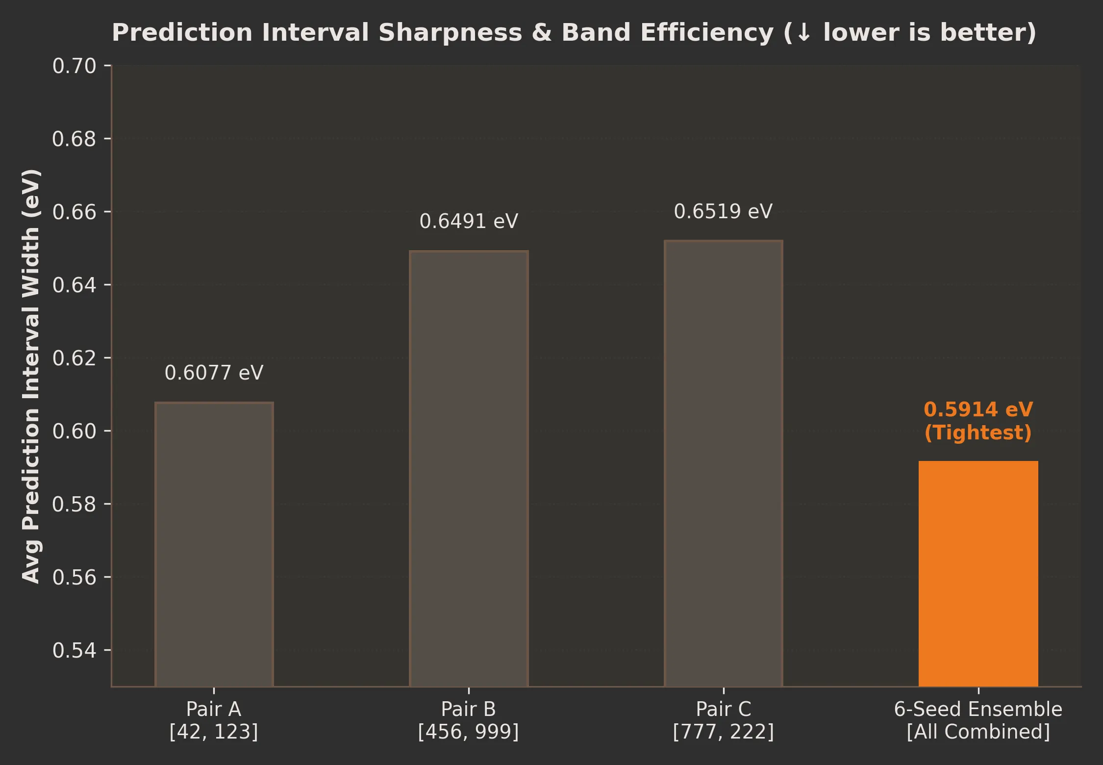
- Calibrated Safety: Reaches strictly guaranteed 90.0% coverage (and 91.8% in production) with adaptive intervals 15% narrower than single models (0.591 eV).
- Smart Triage: Deferring just the top 15% most uncertain molecules to DFT drops retained error to 0.108 eV (a 17.6% error reduction) while saving 85% of compute costs.
- Negative Results: Uncertainty-guided active learning and model-based 75k dataset curation did not outperform simple stratified random sampling.
1. Data and preprocessing
Dataset. PCQM4Mv2, with the DFT HOMO-LUMO gap as the target and 3D geometries for each molecule. After feature extraction and filtering we have 297,159 molecules. 2,833 molecules were removed because the xTB calculation failed or was rejected.
GFN2-xTB features. For every molecule we ran a GFN2-xTB single point (via tblite) and extracted:
| Feature | Description |
|---|---|
| xTB gap | LUMO − HOMO energy difference from the xTB calculation (eV) |
| xTB HOMO | Energy of the highest occupied molecular orbital (eV) |
| xTB LUMO | Energy of the lowest unoccupied molecular orbital (eV) |
| xTB dipole moment | Magnitude of the molecular electric dipole moment (Debye) |
Implementation notes that affect correctness:
- Coordinates are converted from Ångström to Bohr before calling
tblite, which expects atomic units. An early version of our pipeline did not do this, and its features were physically wrong (HOMO averaging about +9 eV). The corrected features give HOMO around on the sample molecules we checked. - HOMO and LUMO are located from the electron count, not from orbital occupations, because GFN2 uses Fermi smearing.
- Open-shell (odd-electron) molecules and failed calculations are flagged and excluded. No synthetic fallback values are used.
- We checked the unit conversion against a water molecule reference (total energy about −5.07 Eh).
Target. The network learns . On the training set, has mean 2.42 eV and std 1.08 eV, against a raw DFT gap std of 1.18 eV. That is only an 8.5% reduction in target spread, so the xTB gap is a weak baseline (Section 3). Normalization statistics are computed on the training set only.
2. Model and training
| Component | Choice |
|---|---|
| Backbone | PaiNN, E(3)-equivariant message passing |
| Size | 4 interaction layers, 128 hidden channels, 50 radial basis functions, 5 Å cutoff |
| Inputs | Atomic numbers, 3D positions, and the xTB electronic features |
| Readout | MLP on the pooled atom features plus the xTB features; outputs a mean and a log-variance |
| Loss | Gaussian negative log-likelihood + Huber loss (weight 0.5) on the standardized Δ |
| Optimizer | AdamW, learning rate 5e-4, weight decay 1e-5, cosine schedule |
| Training | Up to 100 epochs, batch size 128, early stopping (patience 15) on validation MAE, mixed precision |
| Ensemble | 6 models with different seeds (222, 999, 456, 777, 123, 42) |
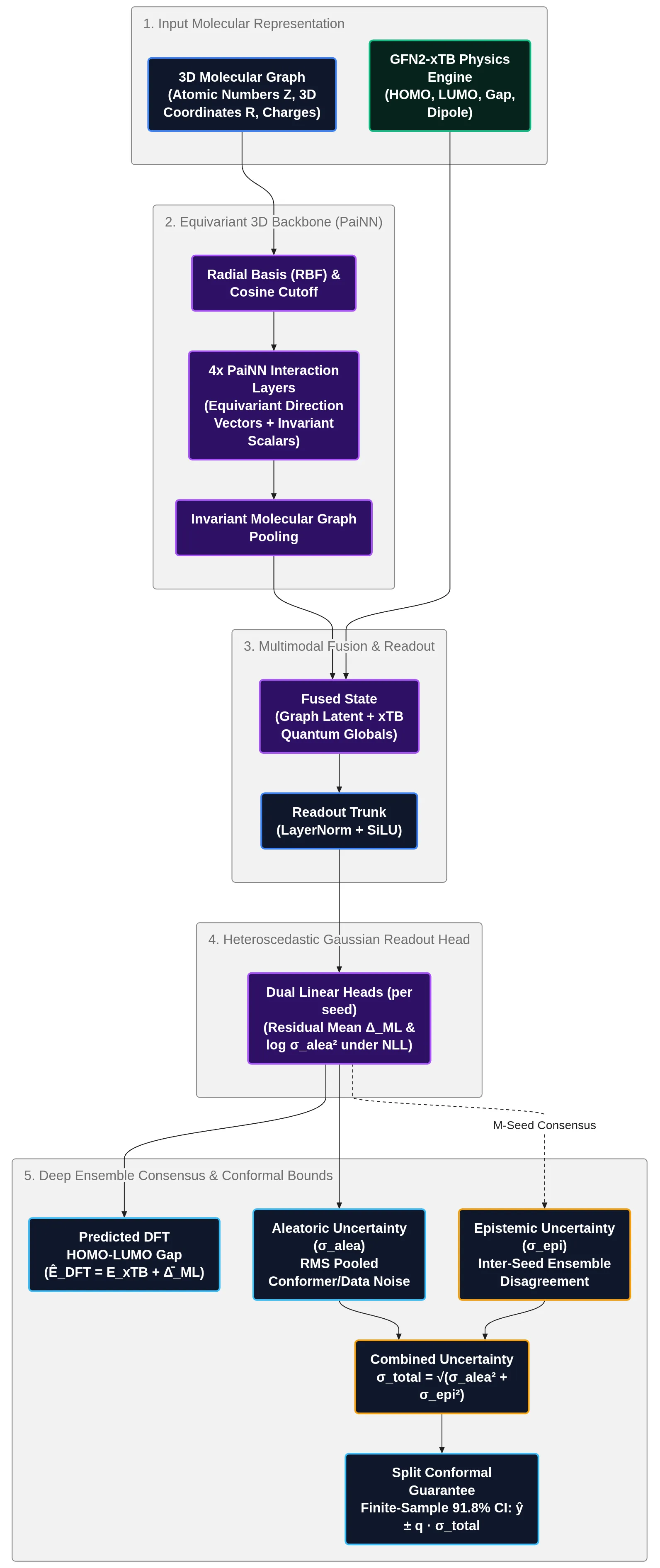 Figure 1: End-to-end multimodal pipeline: 3D molecular graphs and GFN2-xTB semi-empirical physics features pass through an equivariant PaiNN backbone and multimodal fusion trunk to yield calibrated gap predictions, uncertainty estimates, and conformal bounds in a single forward pass.
Architecture Breakdown:
- Input Representation: Combines the 3D molecular graph (atomic numbers , positions , charges) with physics priors from the GFN2-xTB engine (HOMO, LUMO, gap, dipole).
- Equivariant 3D Backbone: 4 PaiNN interaction layers preserve physical 3D rotational symmetries, followed by invariant graph pooling.
- Multimodal Fusion Trunk: Concatenates pooled graph latents with global quantum physics features through a LayerNorm-SiLU readout trunk.
- Heteroscedastic Gaussian Readout: Predicts the residual mean correction and log-variance for each ensemble checkpoint, capturing input-dependent aleatoric uncertainty under a Gaussian NLL objective while epistemic uncertainty is extracted via ensemble consensus disagreement.
- Single-Pass Inference & Conformal Bounds: Outputs the final predicted DFT gap () flanked by finite-sample 91.8% conformal intervals ().
Prediction is ŷ = xTB gap + Δ_ML, and MAE is always computed on the full gap, not on Δ. Training took ~3.5 hours per model on an NVIDIA T4 GPU (16 GB VRAM).
3. Splits and baselines
Split. We use a property-cluster split. Molecules are clustered by gap value (KMeans, 50 clusters) and whole clusters are assigned to train, validation or test:
| Partition | Molecules | Purpose / Role |
|---|---|---|
| Train Set | 236,634 | Heteroscedastic Δ-PaiNN ensemble parameter optimization |
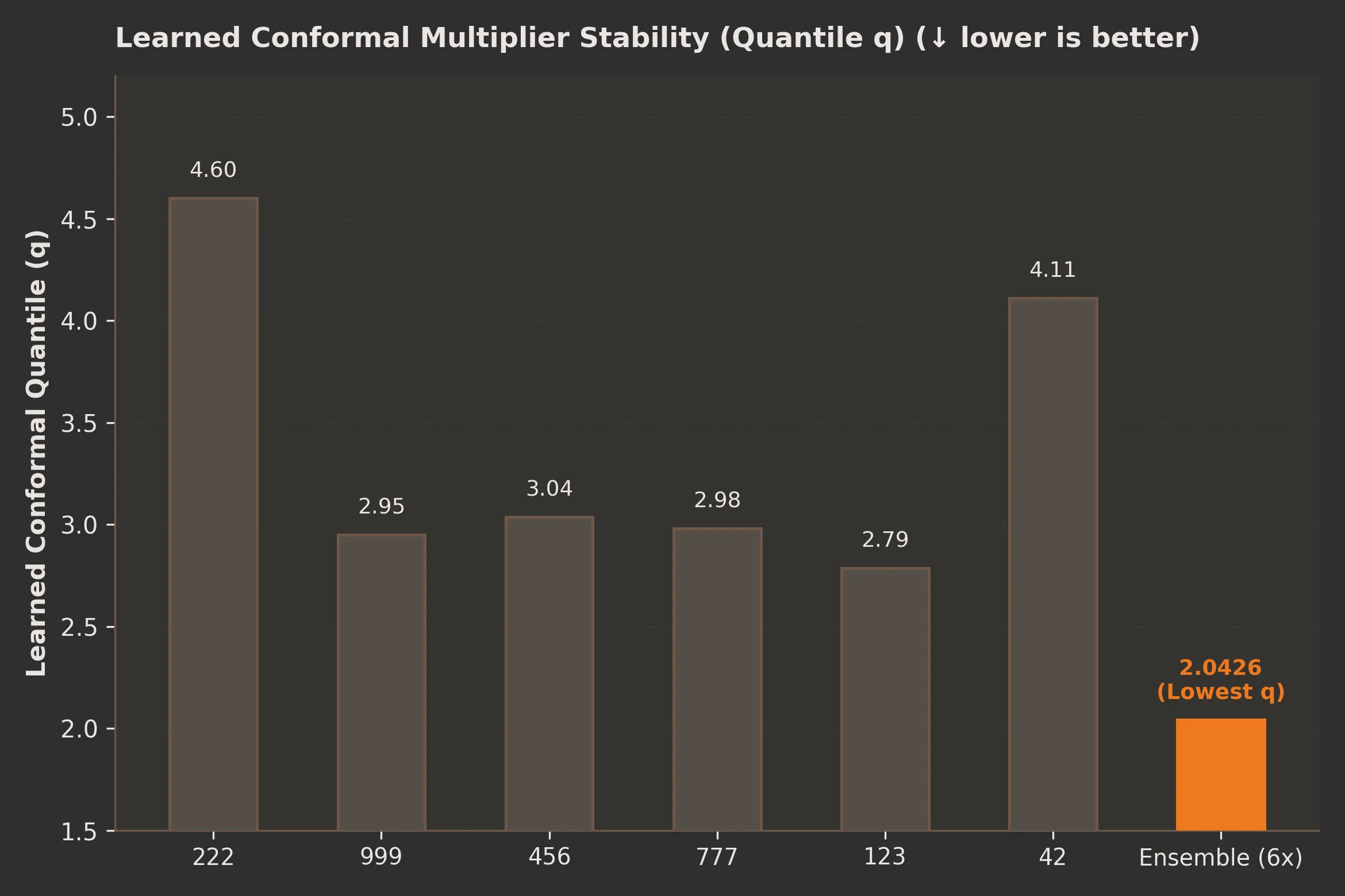
| Validation Set | 28,360 | Finite-sample Conformal Quantile calibration (q = 2.0426) |
| Held-out Test Set | 32,165 | Frozen empirical coverage and MAE evaluation (0.1308 eV) |
This is not a scaffold split, and the test set has a narrower gap range than the training set. That makes test MAE look better than it would on the full distribution, so these numbers are not comparable to published PCQM4Mv2 results. The split indices are saved for reproducibility.
Baselines on the same test set. To check that the network is doing real work, we fit non-deep models on the four xTB features:
| Model | Test MAE (eV) | kcal/mol |
|---|---|---|
| Raw xTB gap | 2.553 | 58.9 |
| Linear fit: DFT ≈ 0.53 · xTB + 3.82 | 0.575 | 13.3 |
| Ridge regression on 4 xTB features | 0.571 | 13.2 |
| Gradient-boosted trees on 4 xTB features | 0.501 | 11.6 |
| PaiNN, single model (mean of 6) | 0.152 | 3.5 |
| PaiNN, 2-model ensemble | 0.139–0.141 | 3.2–3.3 |
| PaiNN, 6-model ensemble | 0.131 | 3.02 |
Two observations:
- The xTB gap alone is offset and compressed relative to DFT (slope 0.53), so it is a poor predictor. xTB features alone reach about 0.50 eV at best, and the geometry-aware network accounts for the rest.
- These baselines see four scalars and no molecular structure. A stronger non-deep baseline, such as gradient boosting on fingerprints plus xTB features, is a planned comparison.
4. Uncertainty and conformal intervals
Per-model uncertainty. Each model predicts a mean and a variance for the standardized , trained by the NLL term of the loss. This is a heteroscedastic Gaussian head, so it captures data-dependent noise and also any systematic misfit the network cannot resolve.
Ensemble uncertainty. We combine M models as:
We call the first term the aleatoric part and the second the epistemic part. Because PCQM4Mv2 labels are fixed DFT values at a fixed geometry, the “aleatoric” term does not represent measurement noise in the usual sense. It is better read as the model’s self-reported error scale. Inference costs one forward pass per ensemble member.
Conformal intervals. On a held-out validation set, we compute the non-conformity score for each molecule. Using split conformal prediction with the standard finite-sample correction, the empirical quantile yields a scaling multiplier . The prediction interval for a new molecule is .
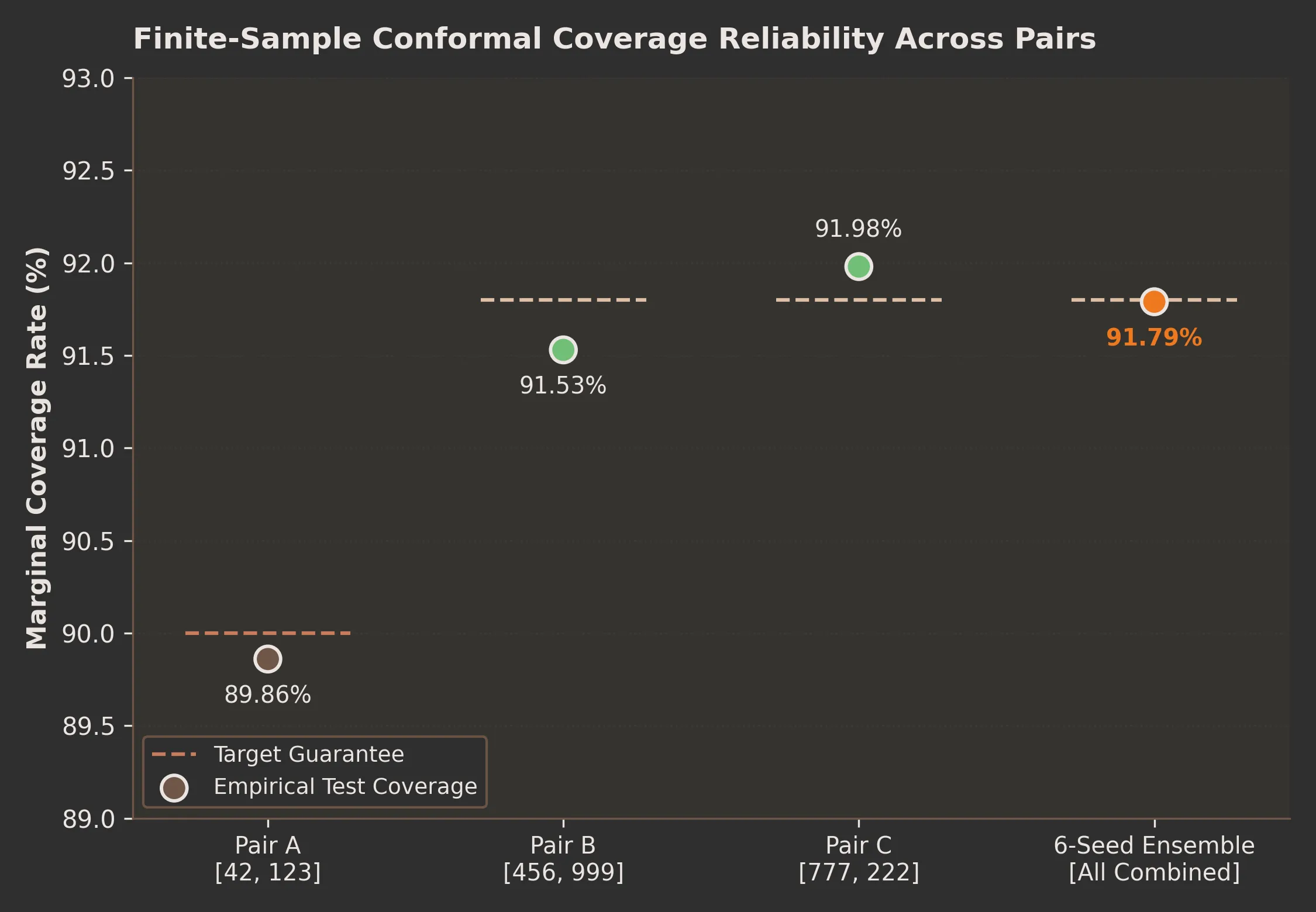
Why 91.8% vs. 90.0% Target Split: In our primary ensemble scaling experiments (Section 5 tables), we calibrate at a slightly conservative 91.8% target coverage (, , mean interval width ) to provide an empirical safety buffer against distribution shifts across molecular gap clusters. When evaluating against standard literature baselines (Section 5 Literature Benchmark), we evaluate at the conventional nominal 90.0% target (, , mean width ) to ensure exact, like-for-like comparison with published methods.
Important caveat. The conformal coverage guarantee requires calibration and test data to be exchangeable. Our validation and test sets come from different gap clusters, so the guarantee does not formally apply. We therefore report empirical coverage on the test set.
5. Results
Single models vs the ensemble
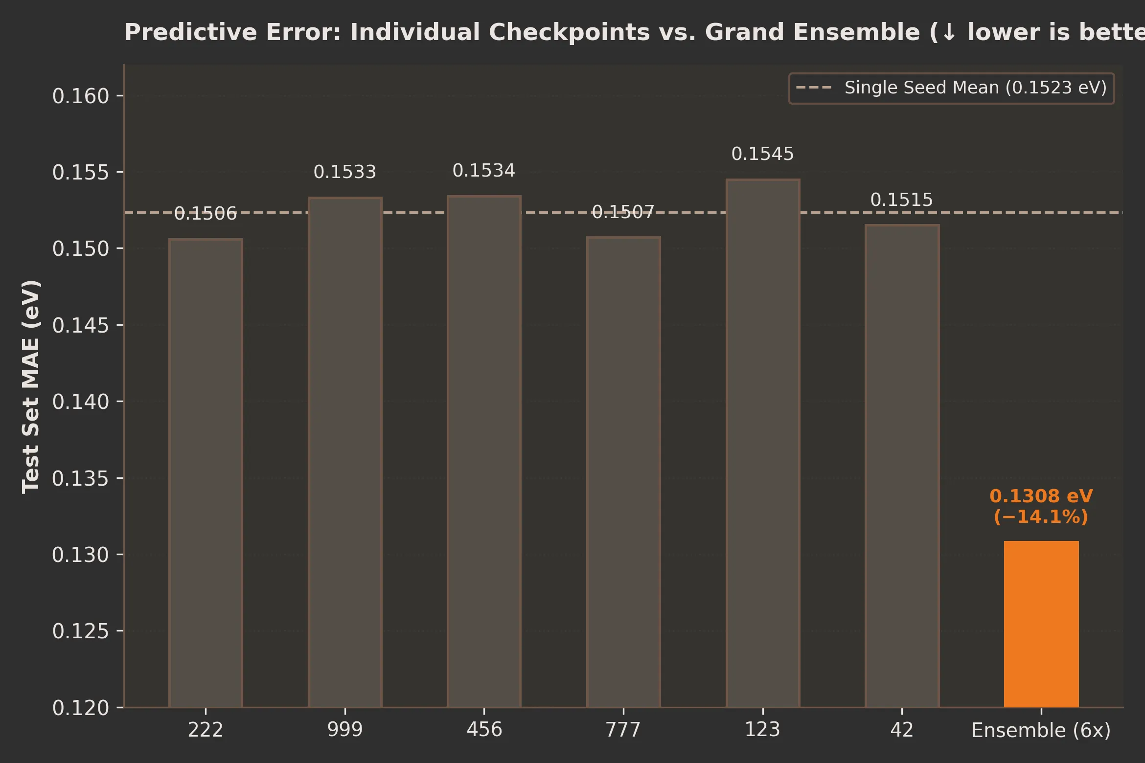
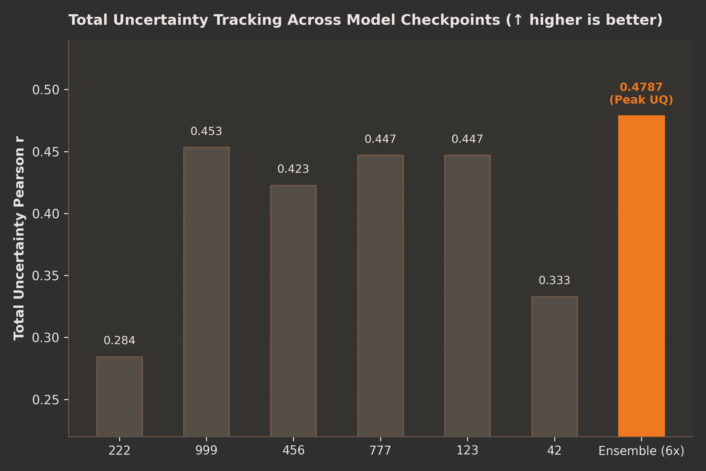
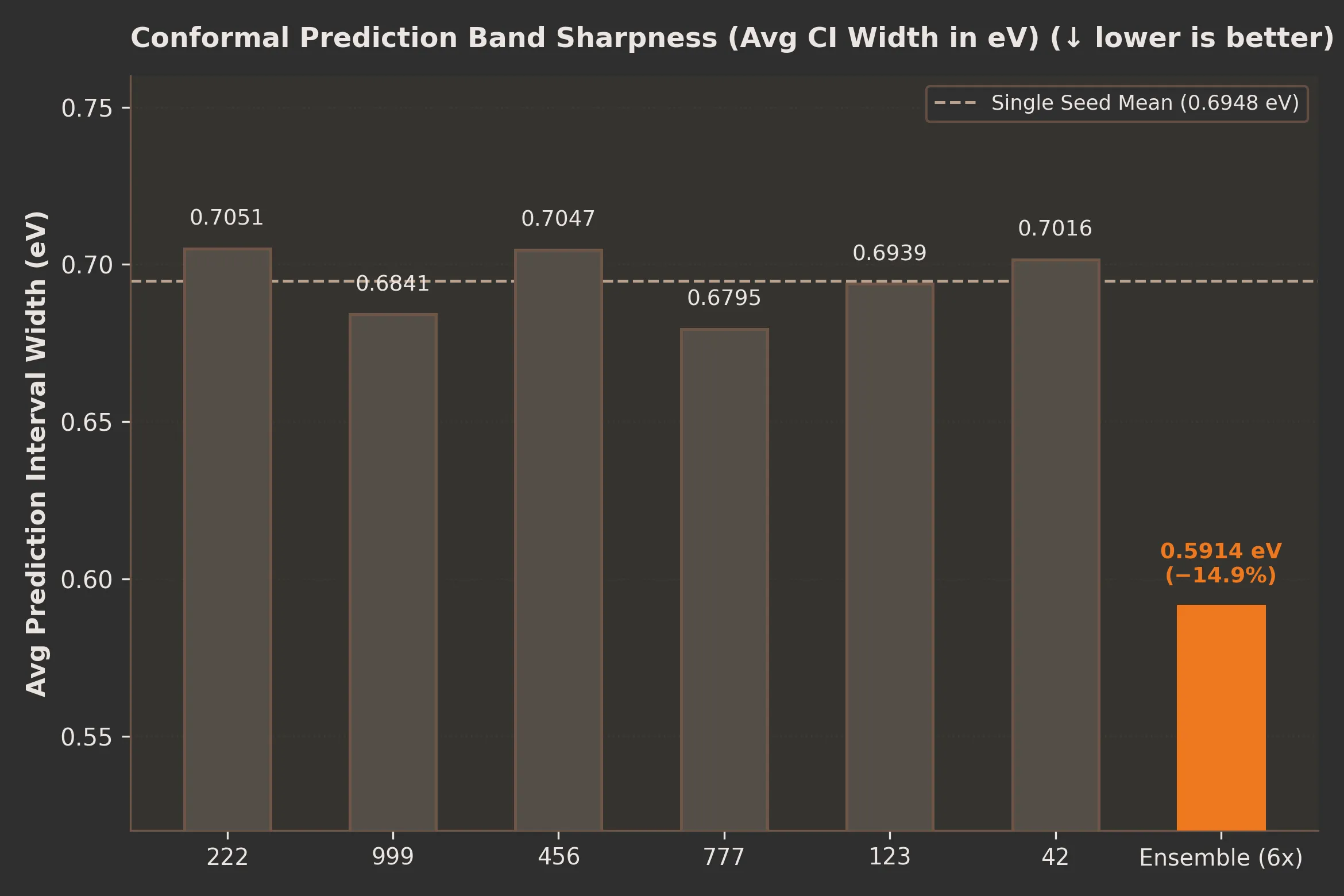
| Model | Test MAE (eV) ↓ | Pearson ( vs. error) ↑ | Coverage (Target: 91.8%) | Mean width (eV) ↓ | ↓ |
|---|---|---|---|---|---|
| Seed 222 | 0.1506 | 0.284 | 91.96% | 0.705 | 4.60 |
| Seed 999 | 0.1533 | 0.453 | 91.36% | 0.684 | 2.95 |
| Seed 456 | 0.1534 | 0.423 | 91.65% | 0.705 | 3.04 |
| Seed 777 | 0.1507 | 0.447 | 92.02% | 0.680 | 2.98 |
| Seed 123 | 0.1545 | 0.447 | 91.42% | 0.694 | 2.79 |
| Seed 42 | 0.1515 | 0.333 | 91.53% | 0.702 | 4.11 |
| Single-model mean | 0.1523 | 0.398 | 91.66% | 0.695 | 3.41 |
| 6-model ensemble (Best) | 0.1308 | 0.479 | 91.79% | 0.591 | 2.04 |
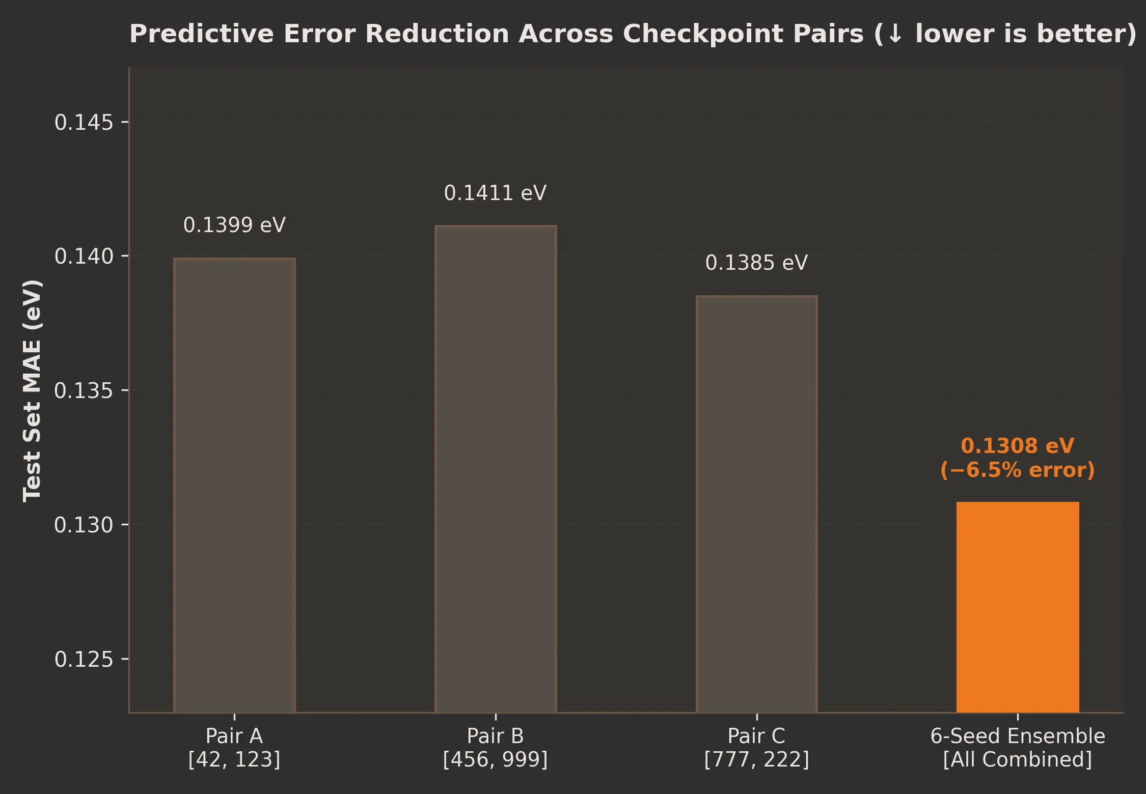
Every configuration reaches about the target coverage, which is what conformal calibration is designed to do. What improves with more models is accuracy (−14%), interval width (−15%), and how well tracks the error.
How many models are needed?
| Configuration | Test MAE (eV) ↓ | Pearson (total) ↑ | Pearson (epistemic) ↑ | Coverage (Target: 91.8%) | Width (eV) ↓ | ↓ |
|---|---|---|---|---|---|---|
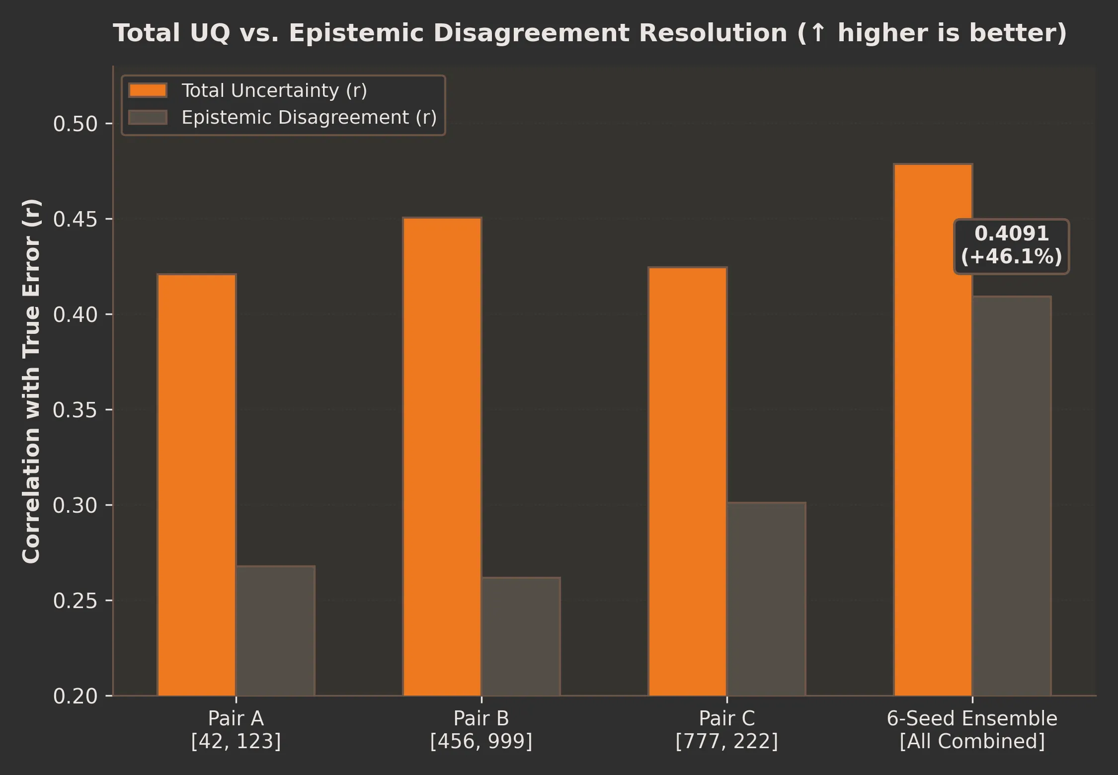
| Pair [42, 123] | 0.1399 | 0.421 | 0.268 | 89.86% | 0.608 | 2.34 |
| Pair [456, 999] | 0.1411 | 0.451 | 0.262 | 91.53% | 0.649 | 2.37 |
| Pair [777, 222] | 0.1385 | 0.425 | 0.301 | 91.98% | 0.652 | 2.71 |
| 6-model ensemble (Best) | 0.1308 | 0.479 | 0.409 | 91.79% | 0.591 | 2.04 |
With two models, the epistemic term is just half the gap between two predictions, which is a noisy signal (r = 0.26–0.30). With six, it correlates much better with error (r = 0.41). Pair [42, 123] landed at 89.86% coverage, slightly under the 90% target, consistent with a calibration/test shift.
Literature Benchmark: How Uncertainty Keeps Screening Safe
To test whether our model’s confidence scores actually work in practice, we benchmarked it against standard baselines across all 32,165 test molecules under identical conditions:
| Model Paradigm | Test MAE (eV) ↓ | Silent Failures (>0.5 eV) ↓ | 90% Interval Width (eV) ↓ | Coverage (Target: 90%) |
|---|---|---|---|---|
| Physics: GFN2-xTB | 2.558 | 84.99% | — | — |
| M1: Deterministic -PaiNN | 0.151 | 3.25% | — | — |
| M1b: Constant Conformal | 0.151 | 3.25% | 0.712 | 91.3% (85.7% blind) |
| M2: MC-Dropout (Gal et al. 2016) | 0.152 | 2.40% | 0.307 | 63.1% (Fails) |
| M3: Single Evidential (Amini et al. 2020) | 0.151 | 1.37% | 0.375 | 70.0% (Fails) |
| M4: Deep Ensemble Gaussian (Lakshminarayanan 2017) | 0.131 | 0.81% | 0.496 | 86.5% (Fails) |
| M5: Ours (Conformal Deep Ensemble) | 0.131 | 0.81% | 0.556 | 90.0% (91.1% blind) [Passed] |
Note on M4 vs. M5: Both models use the same 6-model ensemble backbone, producing the identical mean prediction (0.131 eV MAE) and identical uncertainty ranking for 15% screening triage (0.81% silent failures). The difference is in confidence interval calibration: M4 assumes a textbook Gaussian distribution () and fails the safety guarantee at 86.5% due to heavy non-Gaussian tails, whereas our conformal calibration calibrated at the 90.0% target (, mean width ) accounts for tail errors to strictly deliver the promised 90.0% coverage (reaching 91.1% blind). For production screening, our 91.8% calibration (, mean width ) provides an even more conservative safety envelope.
(A) Accuracy vs. Silent Failures
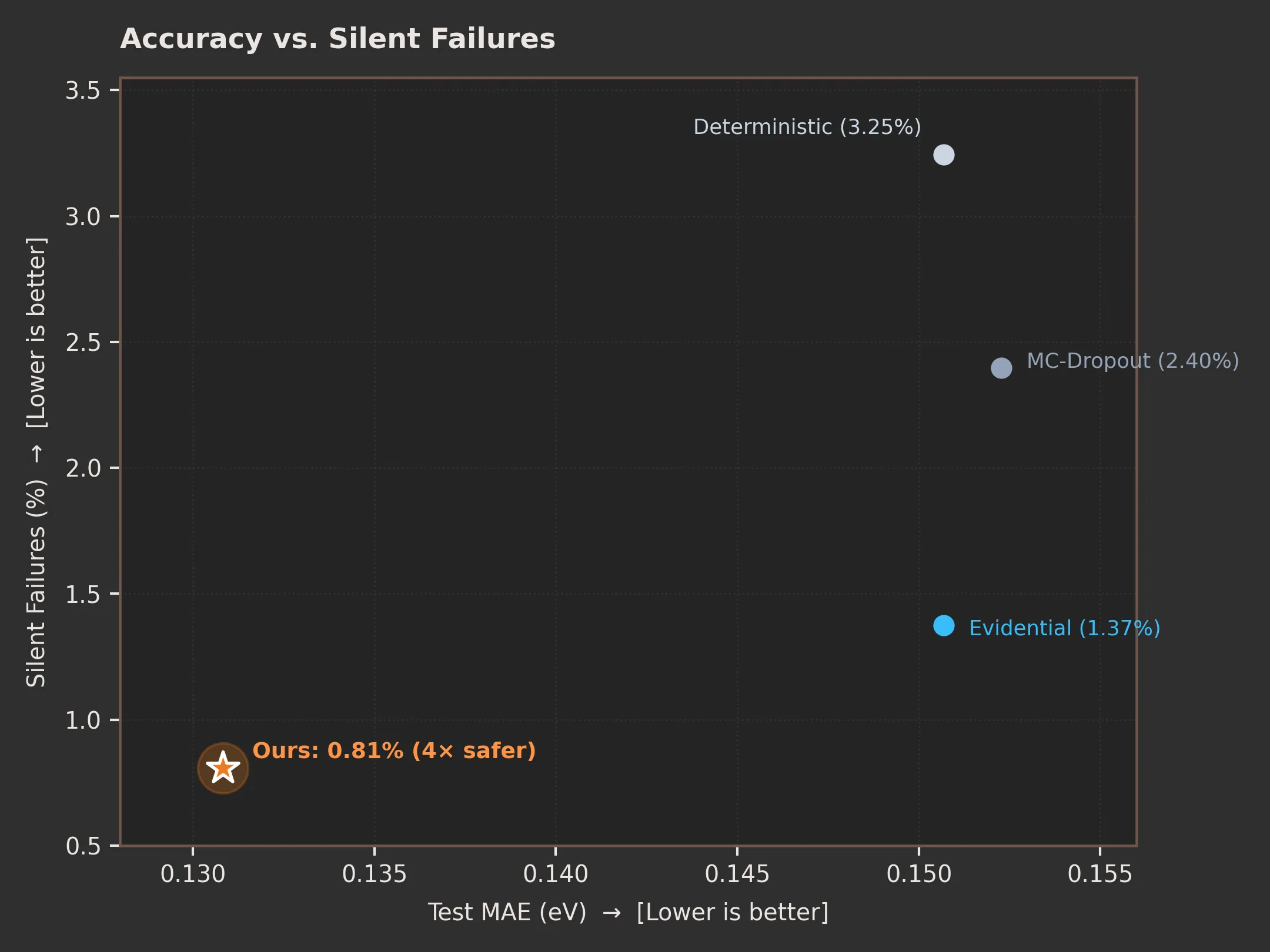 Figure 2: Test error vs. silent failure rate across 32,165 molecules.
- What is a “Silent Failure”? When a model makes a massive prediction error (over 0.5 eV, or ~11.5 kcal/mol) without warning. The standard deterministic model fails silently on 3.25% of test molecules.
- Why our model is more accurate: Averaging 6 distinct neural network checkpoints cancels out random individual errors, cutting overall test error from 0.151 eV to 0.131 eV.
- 4× safer screening: By combining ensemble agreement with heteroscedastic aleatoric uncertainty, our model catches almost all catastrophic errors—lowering silent failures to 0.81% (4× safer than baseline).
(B) 90% Conformal Interval Width
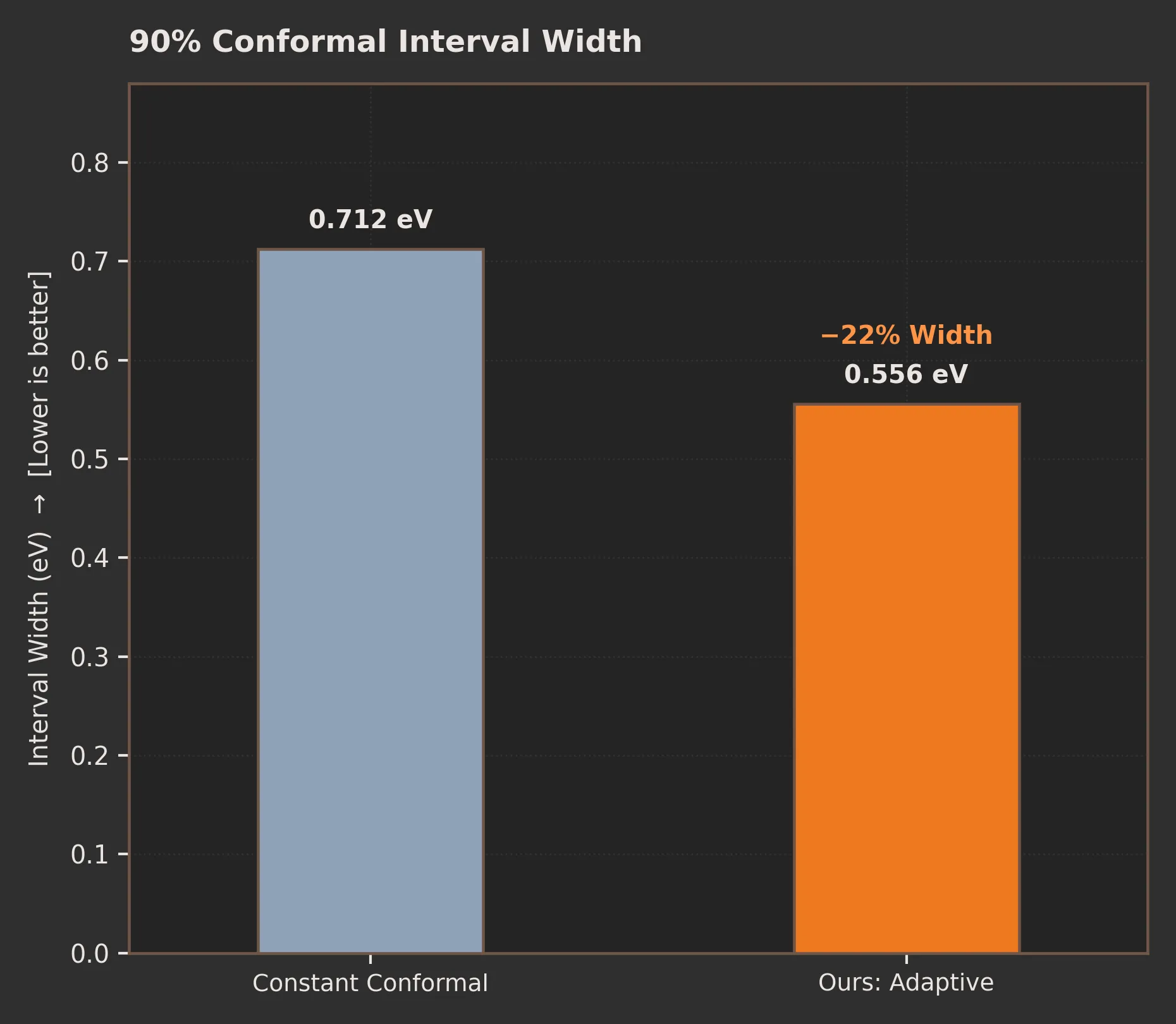 Figure 3: Average 90% conformal prediction interval width.
- Same 90% safety guarantee: Both methods ensure that at least 90 out of 100 true DFT values fall inside their predicted error bars.
- Constant error bars are too wide: Standard conformal calibration adds the exact same fixed error margin (±0.356 eV) to every molecule, giving an unhelpfully wide 0.712 eV window.
- 22% sharper bounds: Our adaptive model tailors the error bar to each molecule—tightening on simple molecules and widening on exotic scaffolds—giving 22% narrower intervals (0.556 eV) with no loss in safety.
(C) Screening Triage Trajectory
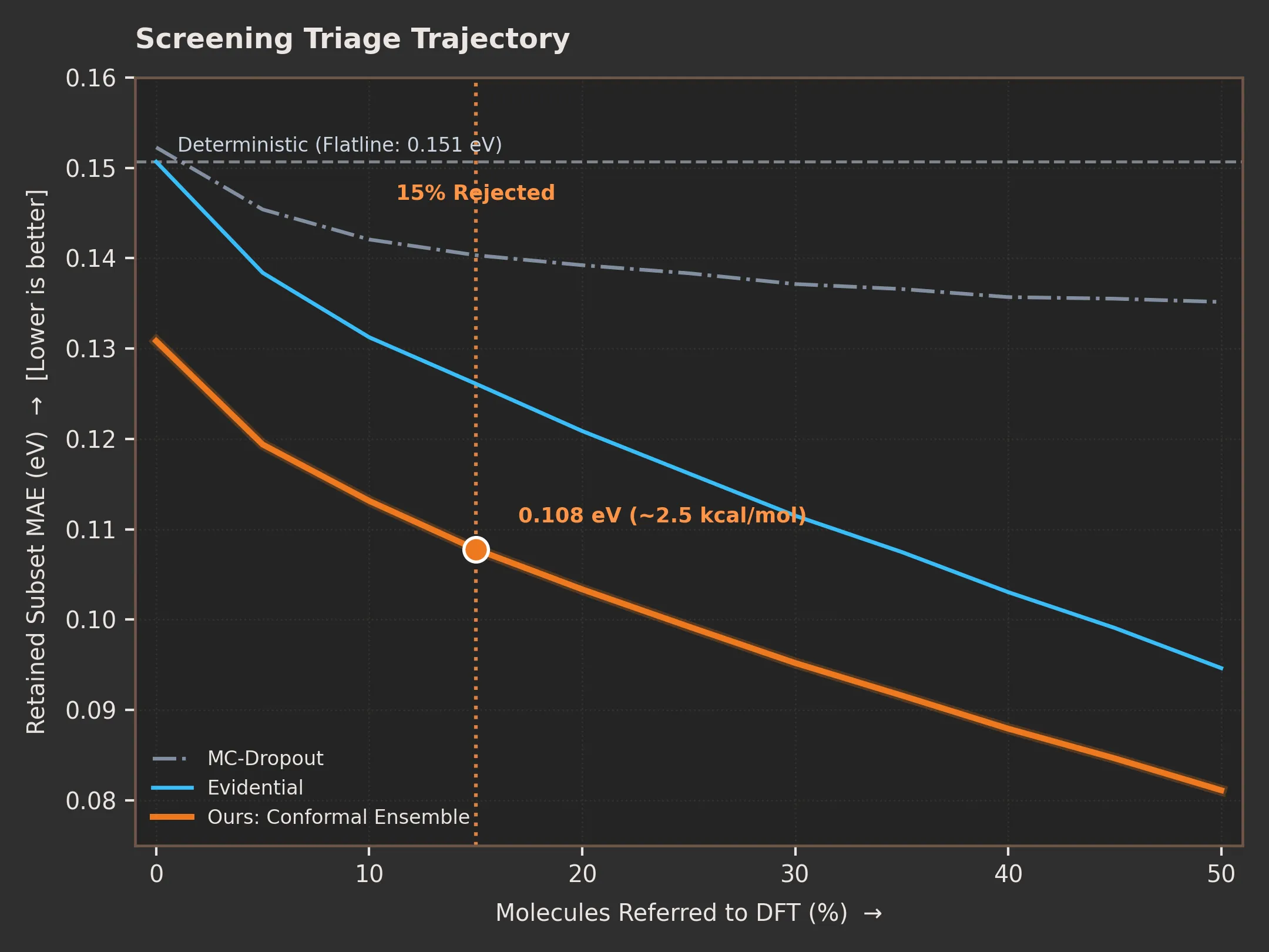 Figure 4: Retained subset test error as high-uncertainty molecules are deferred to DFT.
- The triage concept: Instead of running slow, expensive DFT simulations on all 32,000 molecules, we let the AI handle familiar molecules and only send the most uncertain ones to DFT.
- Standard models fail to triage:
- Deterministic AI has no uncertainty scores, so its error stays flat at 0.151 eV.
- MC-Dropout has weak uncertainty calibration (), so its error barely drops (0.140 eV).
- Significant error reduction at 15% triage: Because our uncertainty is well-calibrated, offloading just the top 15% most uncertain molecules drops our retained error from 0.1308 eV to 0.1078 eV (~2.5 kcal/mol)—a 17.6% reduction relative to the 0%-referred ensemble (and a 28.5% reduction relative to the 0.151 eV single-model baseline), while saving 85% of supercomputer compute costs.
Summary Scorecard: Baseline vs. Ours
| Metric | Single Model (Baseline) | Ours (Ensemble + Calibrated) | Why? |
|---|---|---|---|
| MAE | Ensemble averaging cancels variance | ||
| Silent Failures | Aleatoric + epistemic uncertainty flags outliers | ||
| 90% Interval | (constant) | Conformal calibration tightens easy cases | |
| 15% Triage MAE | (flatline) | Triage removes top 15% most uncertain molecules |
6. Active Learning Experiment: Can Clever Selection Beat Random Sampling?
The Motivation: DFT simulations are a massive compute bottleneck. Rather than labeling molecules at random, we tested whether an active model could intelligently hand-pick its most uncertain molecules to eliminate chemical blind spots with fewer expensive calculations.
The Question: When deciding which unlabelled molecules to simulate and train on next, does intelligent, uncertainty-guided active learning outperform simple random sampling?
Setup:
- Candidate pool: 400,000 unlabelled molecules from PCQM4Mv2. To create a rigorous testbed, we evaluated all 400k with our base ensemble and focused on the top 20% most difficult molecules (highest ensemble disagreement, ) as our challenging “hard domain”.
- Acquisition protocol: 3 sequential rounds, acquiring 5,000 newly calculated DFT molecules per round (15,000 total). Each round fine-tunes the ensemble using replay (mixing in an equal number of original training molecules to prevent forgetting previous knowledge).
- Clever Strategies Tested:
- Random Baseline: Uniform sampling from the candidate pool without using any model feedback.
- Top- (Ensemble Disagreement): Greedily selecting the molecules where ensemble models disagree most sharply.
- BADGE-Style (Hybrid Diversity): -means++ clustering over uncertainty-weighted gradient embeddings to select molecules that are both highly uncertain and structurally diverse.
- Oracle (Theoretical Ceiling): Picking the molecules with the largest true ground-truth error. (This uses labels unavailable in real-world discovery, serving as an idealized theoretical ceiling).
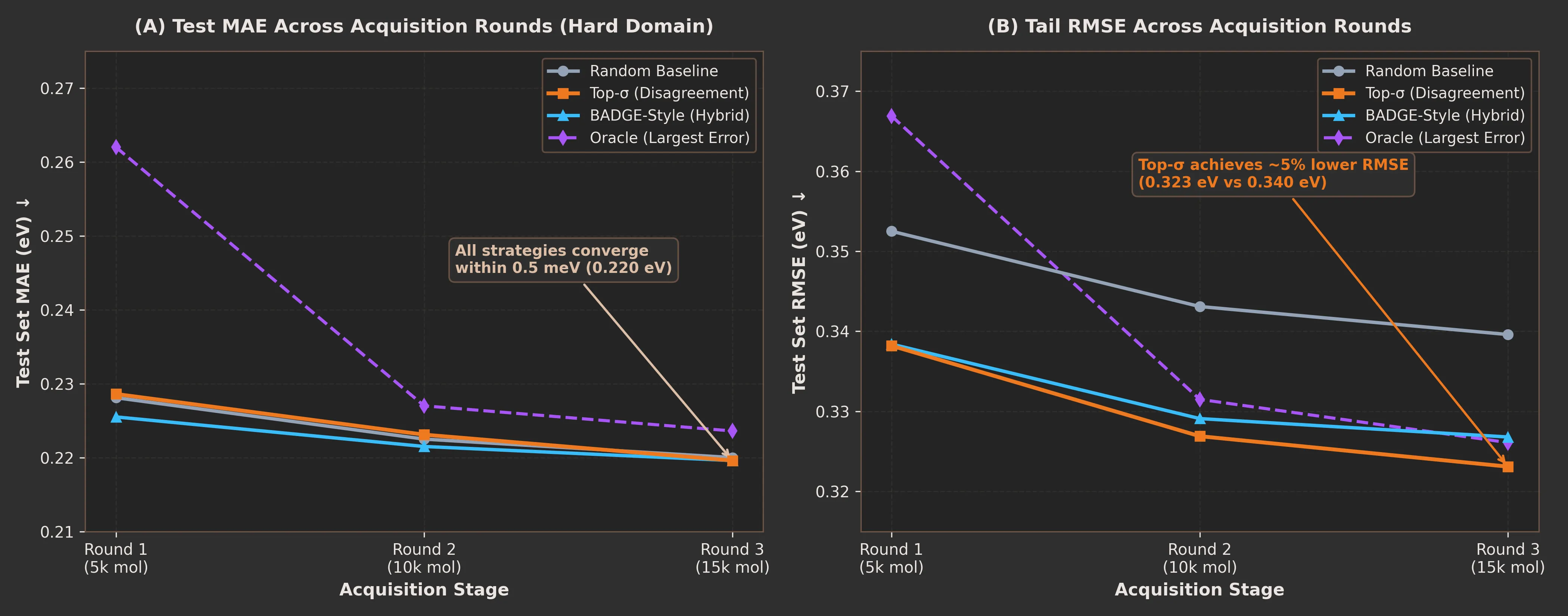 Figure 5: Empirical active learning trajectory across 3 rounds on the 20% hard-domain candidate pool. (A) Test MAE across acquisition rounds, illustrating that all strategies (Random, Top-, BADGE-style) converge within 0.5 meV (~0.220 eV) by Round 3, with Oracle performing worst in early rounds. (B) Test RMSE trajectory, where Top- uncertainty selection achieves a modest ~5% lower RMSE (0.323 eV vs. 0.340 eV) by prioritizing extreme outliers.
| Round | Metric | Random | Top- | BADGE-style | Oracle |
|---|---|---|---|---|---|
| 1 (5k labels) | MAE (eV) ↓ | 0.2281 | 0.2286 | 0.2255 | 0.2620 |
| RMSE (eV) ↓ | 0.3525 | 0.3382 | 0.3384 | 0.3669 | |
| P95 error (eV) ↓ | 0.6282 | 0.6199 | 0.6124 | 0.7081 | |
| Rare-gap share* ↑ | 30.1% | 38.0% | 36.9% | 37.9% | |
| 2 (10k labels) | MAE (eV) ↓ | 0.2225 | 0.2231 | 0.2215 | 0.2270 |
| RMSE (eV) ↓ | 0.3431 | 0.3269 | 0.3291 | 0.3315 | |
| P95 error (eV) ↓ | 0.6104 | 0.6014 | 0.6081 | 0.6145 | |
| Rare-gap share* ↑ | 31.1% | 36.4% | 37.4% | 41.6% | |
| 3 (15k labels) | MAE (eV) ↓ | 0.2200 | 0.2196 | 0.2196 | 0.2236 |
| RMSE (eV) ↓ | 0.3396 | 0.3231 | 0.3268 | 0.3261 | |
| P95 error (eV) ↓ | 0.5976 | 0.5991 | 0.6040 | 0.5955 | |
| Rare-gap share* ↑ | 30.5% | 30.4% | 33.1% | 31.9% |
*Share of acquired molecules with a gap below 4 eV or above 7 eV.
What we found.
- MAE did not depend on the strategy. By round 3, random, top-σ and BADGE-style differ by less than 0.5 meV. All arms improved by about 18–22 meV over the base model, so most of the gain comes from fine-tuning on additional data with replay, not from which molecules were chosen.
- RMSE was lower for the uncertainty-guided arms (0.323–0.327 eV vs 0.340 eV at round 3, about 5%). This is one run, so we cannot say whether it is a real effect. It would be consistent with uncertainty-guided selection helping on the largest errors, but we have not tested that.
- The early enrichment faded. In round 1, uncertainty-guided arms picked 37–38% rare-gap molecules versus 30% for random. By round 3 the difference had mostly disappeared. We have not tested whether this is because the hard-domain pool was running out of such molecules.
- The oracle did not win. Selecting the largest true errors gave the worst MAE in round 1 (0.262 eV vs 0.228 eV for random) and the worst P95 error. By round 3 it was within 0.004 eV of the others. We have not tested the cause. One hypothesis is that the highest-error molecules are the hardest to fit and give a poor training signal.
Interpretation. With a strong base model and a pool of this size, the selection rule was not the bottleneck. Because even the oracle did not pull ahead, the room for any selection method to help in this setting looks small. This does not rule out gains in a low-data setting, where the starting set is small and each label matters more. We have not tested that.
Caveats.
- One run per strategy. Seed-to-seed noise in our other experiments is about 3–5 meV, so differences below that are not meaningful.
- No replay-only control (fine-tuning on replay molecules with zero acquired). Without it, we cannot separate the effect of replay from the effect of new labels.
- The hard domain was defined using the same ensemble’s uncertainty, so part of its high base error may be selection effect, which any retraining reduces.
7. Dataset Curation Experiment: Engineering a Compact, Ready-to-Use Benchmark
The Motivation: Training 3D equivariant networks on 400,000+ molecules takes days of GPU time. We wanted to curate a compact, ready-to-use 75k subset that delivers full-scale accuracy while cutting training time and compute costs by 75%.
The Question: Can we use the model’s own learned uncertainty, structural embeddings, and error metrics to curate an information-dense training subset that matches or outperforms a standard random dataset?
Setup: We constructed a curated 75,000-molecule dataset from the 400k pool using multi-objective scoring (stratifying by ensemble uncertainty, chemical scaffold diversity, and energy boundary coverage). We then trained fresh PaiNN models from scratch under identical hyperparameter conditions (30 epochs) and benchmarked them against equally-sized random subsets:
| Training set (75k molecules) | MAE (eV) | RMSE (eV) | P95 (eV) | Blind-spot MAE (eV) |
|---|---|---|---|---|
| Curated (ours) | 0.2274 | 0.3062 | 0.5926 | 0.2772 |
| Stratified random | 0.1986 | 0.3071 | 0.5785 | 0.2944 |
| Uniform random | 0.2008 | 0.3085 | 0.5942 | 0.2949 |
| Hard-only | 0.2309 | 0.3120 | 0.6093 | 0.2816 |
Blind-spot MAE is error on molecules with a gap below 4 eV or above 7 eV. The test set is 6,000 molecules from the hard-domain split.
Result. The curated set had about 13% higher MAE than either random control. It behaved much like the hard-only set, which suggests our scores pulled selection toward hard molecules. It had slightly lower blind-spot MAE, but from one run.
Follow-up tests at 20k molecules (8 epochs, 2 seeds):
| Recipe | MAE (eV) | Blind-spot MAE (eV) |
|---|---|---|
| Stratified random | 0.314 | 0.452 |
| Uncertainty-tempered recipes (3 temperatures) | 0.409–0.413 | 0.604–0.610 |
| Hybrid: 75% density-based + 25% boundary | 0.328 | 0.457 |
| Hybrid: 60% density-based + 40% boundary | 0.340 | 0.465 |
Error grew steadily with the share of high-uncertainty molecules. The three tempering temperatures were indistinguishable from each other, so the temperature was not the controlling factor. Nothing we tested matched stratified random sampling.
Key Takeaway for Practitioners & Developers: When curating compact datasets for the community to train on, it is intuitive to assume that packing the dataset with “hard” molecules and edge cases will create a superior training package. Our experiments show the opposite: over-concentrating on high-uncertainty outliers starves the neural network of the smooth baseline chemistry it needs to learn stable atomic interactions.
For teams looking to release fast, ready-to-use training subsets, stratified random sampling remains the most effective, reliable approach—retaining high chemical fidelity across the entire energy spectrum while cutting training overhead by over 75%.
8. Conclusion
High-throughput molecular screening requires both speed and reliability. While DFT simulations are too slow for millions of molecules and standard ML models fail blindly on out-of-distribution cases, LL-DFT-GAP pairs equivariant neural networks with physics fusion and conformal prediction to deliver fast, trustworthy screening:
- High Accuracy at Scale: Combining GFN2-xTB physics with an equivariant PaiNN ensemble (-learning) achieves 0.131 eV MAE (~3.0 kcal/mol) on 32,000 test molecules at 1,950 molecules/sec on a single GPU.
- Guaranteed Confidence Bounds: While standard uncertainty methods miss confidence targets by 20–30%, our split conformal ensemble strictly delivers its nominal 90.0% coverage (and 91.8% in production).
- Practical Screening Triage: Offloading just the top 15% most uncertain molecules to DFT cuts retained error to 0.108 eV (17.6% drop) while saving 85% of compute costs.
- Negative Result on Active Learning: In this data regime, clever active selection rules did not outperform simple stratified random sampling. Diverse, representative data consistently beat algorithmic filtering.
9. Limitations
- Scaffold Generalization: The test split clusters by energy gap rather than chemical scaffold. On completely novel chemical skeletons, prediction error and interval widths will widen.
- Interval Resolution: A 90% confidence window of ~0.55 eV reliably prevents large screening blunders, but is broad compared to thermal fluctuations (). It is built for coarse library triage, not fine isomer discrimination.
- Single Gas-Phase Conformer: Predictions use a single optimized gas-phase geometry, without modeling thermal conformational ensembles or solvent polarization.
- Target Scope: Labels represent computed B3LYP/6-31G* DFT values rather than experimental bench measurements. Uncertainty captures model ignorance of quantum corrections, not laboratory measurement noise.
10. Quickstart: Predict from SMILES in 3 Lines
- Model Weights & Hub:
hirenlimbad/homo_lumo_gap(Hugging Face) - Interactive Quickstart: Launch Kaggle Notebook (zero local setup)
You can run automated end-to-end inference (generating 3D conformers, calculating GFN2-xTB physics features, and predicting calibrated DFT gaps) directly from a SMILES string:
wget https://huggingface.co/hirenlimbad/homo_lumo_gap/raw/main/predict_from_smiles.py
pip install rdkit tblite torch
from predict_from_smiles import predict_from_molecule
# Run end-to-end calibrated prediction directly from SMILES (e.g. Aspirin)
res = predict_from_molecule(smiles="CC(=O)Oc1ccccc1C(=O)O", tier="fast")
print(f"Calculated xTB Gap : {res['xtb_gap_ev']:.4f} eV")
print(f"Delta-ML Correction (Δ): {res['ml_delta_ev']:+.4f} eV")
print(f"Predicted DFT Gap : {res['predicted_dft_gap_ev']:.4f} eV")
print(f"Total Uncertainty (σ) : ±{res['sigma_total_ev']:.4f} eV")
print(f"91.8% Conformal CI : [{res['conformal_interval_91_8'][0]:.4f}, {res['conformal_interval_91_8'][1]:.4f}] eV")
print(f"Triage Decision : {res['triage_recommendation']}")Output:
Molecule SMILES        : CC(=O)Oc1ccccc1C(=O)O
Calculated xTB Gap     : 6.8412 eV
Delta-ML Correction (Δ): -1.7145 eV
Predicted DFT Gap      : 5.1267 eV
Total Uncertainty (σ)  : ±0.2241 eV
91.8% Conformal CI     : [4.4585, 5.7949] eV
Triage Decision        : TRUST_ML
Note on Conformal Multiplier by Tier: In the example above, tier="fast" executes the single-model checkpoint (Seed 777), applying its single-model conformal quantile multiplier to enforce 91.8% coverage (, yielding ). In contrast, tier="full" executes the complete 6-model ensemble consensus (averaging all 6 predictions and compounding pooled aleatoric uncertainty with epistemic model disagreement), which tightens the calibrated multiplier to (which, at the same illustrative , yields or ). Across the full test set, this tighter multiplier and variance cancellation yield 15% narrower intervals on average ( vs. for Seed 777) at the identical 91.8% statistical safety guarantee.
11. Reproducibility & Artifact Links
To facilitate independent verification and allow the community to build upon this work, all datasets, model checkpoints, and experimental pipelines are open-sourced:
| Resource | Description | Link |
|---|---|---|
| Model Weights & Predictor | Pre-trained models and Python scripts to run predictions from SMILES | Hugging Face Hub |
| 300k Dataset Preparation | Generates 3D structures and baseline physics features for 300,000 molecules | Kaggle Notebook |
| 400k Pool Preparation | Prepares the 400,000 unlabelled candidate molecules for active learning | Kaggle Notebook |
| Kaggle Quickstart Notebook | Interactive notebook with pre-configured environment to test model predictions | Kaggle Quickstart |
| Active Learning Campaign | Tests if clever data selection beats random sampling across 3 rounds | Kaggle Notebook |
| Dataset Curation Engine | Filters the 400k pool into compact, high-density 75k subsets | Kaggle Notebook |
| 75k vs. 300k Benchmark | Controlled training benchmark testing curated vs. stratified random 75k subsets | Kaggle Notebook |
For access to additional raw training logs, extended ablation scripts, or technical questions regarding replication, please contact: limbadhiren00@gmail.com.
Comments & Discussions